Compare Learning Curves

Assumptions

1. Predefined Dataset Split: A train/test split has already been performed, and the focus is on analyzing the training dataset.
2. Model and Metric: A single machine learning model and performance metric (e.g., accuracy, RMSE, F1 score) have been chosen for evaluation.
3. Learning Curve Analysis: The procedure assumes the goal is to evaluate performance trends as the training set size varies.

Procedure

1. Prepare Training Subsets

   • What to do: Create subsets of the training dataset with varying sizes (e.g., 10%, 20%, 50%, 100% of the data).
   • Why: To observe how model performance changes as the training dataset grows.

2. Perform K-Fold Cross-Validation

   • What to do: For each subset, use k-fold cross-validation to evaluate the model.
     • Record the train and validation performance metrics for each fold.
   • Why: To ensure reliable estimates of performance for each training size.

3. Calculate Average Scores

   • What to do: Compute the average train and validation scores for each training set size.
   • Why: Summarize the performance trends across folds.

4. Plot Learning Curves

   • What to do: Plot a validation curve with:
     • X-axis: Training set size.
     • Y-axis: Train and validation performance scores.
   • Why: To visualize performance trends and diagnose potential overfitting or underfitting.

5. Analyze Trends

   • What to do: Look for key patterns in the learning curve:
     • Does performance improve with more data?
     • Is there a significant gap between train and validation scores?
   • Why: To identify signs of overfitting, underfitting, or appropriate model scaling.

Interpretation

Outcome

• Results Provided:
  • A learning curve plot showing train and validation performance against training set size.
  • Quantitative insights into how the model scales with more data.

Healthy/Problematic

• Healthy Trends:
  • Validation performance improves as training set size increases and stabilizes near train performance, indicating the model generalizes well.
  • A small, narrowing gap between train and validation performance scores as training size increases is expected.
• Problematic Trends:
  • Overfitting: A large gap where train performance is high, but validation performance remains low, even with larger datasets.
  • Underfitting: Both train and validation performance scores remain low and do not improve significantly with more data.
  • Data Issues: Performance does not improve with larger data sizes, suggesting poor data quality or an inappropriate model choice.

Limitations

• Computational Costs: Performing k-fold cross-validation for multiple training set sizes can be time-intensive for large datasets.
• Data Availability: Results may not be meaningful for datasets with insufficient data for incremental subsets.
• Single Metric Focus: Analysis is limited to the chosen performance metric; using multiple metrics may provide a more comprehensive evaluation.
• Simplistic Analysis: Does not account for other factors like feature importance, model complexity, or hyperparameter tuning.

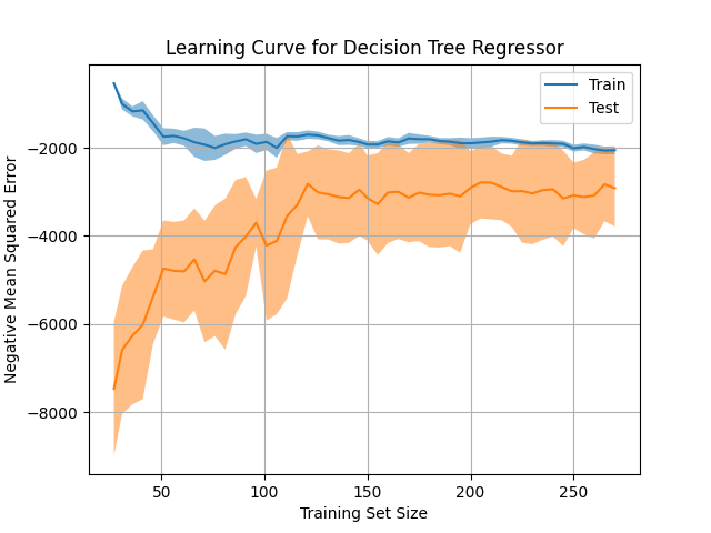
Code Example

This example demonstrates how to use LearningCurveDisplay.from_estimator to automatically calculate and plot a learning curve for a regression task, detecting overfitting or underfitting patterns.

import matplotlib.pyplot as plt
import numpy as np
from sklearn.datasets import make_regression
from sklearn.tree import DecisionTreeRegressor
from sklearn.model_selection import LearningCurveDisplay

# Generate synthetic regression data
X, y = make_regression(n_samples=300, n_features=5, noise=0.1, random_state=42)

# Define a model
model = DecisionTreeRegressor(max_depth=3)

# Plot learning curve using LearningCurveDisplay
disp = LearningCurveDisplay.from_estimator(
    model,
    X,
    y,
    train_sizes=np.linspace(0.1, 1.0, 50),
    cv=10,
    scoring="neg_mean_squared_error",
    score_type="both",
    score_name="Mean Squared Error",
)
disp.ax_.set_title("Learning Curve for Decision Tree Regressor")
disp.ax_.set_xlabel("Training Set Size")
disp.ax_.set_ylabel("Negative Mean Squared Error")
plt.grid(True)
plt.show()

Example Output

Key Features

• Uses LearningCurveDisplay.from_estimator: Automates the calculation and visualization of learning curves with minimal code.
• Variable-Capacity Model: Demonstrates potential overfitting patterns using a model with variable capacity (e.g., DecisionTreeRegressor with max_depth).
• Cross-Validation Built-In: Efficiently calculates learning curves using k-fold cross-validation.
• Automatic Visualization: Provides a clear, annotated plot for both train and validation performance metrics.
• Customizable Configuration: Supports various model types, training sizes, metrics, and cross-validation settings.
• Simplified Workflow: Eliminates the need for manual calculations or separate plot construction, focusing on rapid diagnostics.