Compare Loss Curves

Assumptions

1. Predefined Train/Test Split: Assume the data has already been split into training and testing sets.
2. Model and Metric: A single machine learning model and performance metric (e.g., loss, accuracy, F1 score) have been chosen for evaluation.
3. Model Update Capability: The model provides a mechanism for evaluation after each update, such as training epochs or boosting iterations.

Procedure

1. Train the Model with Evaluation After Each Update

   • What to do: Train the model on the training set and evaluate it on both the training and validation subsets after each update (e.g., epoch, boosting round).
   • Data Collection: Record the performance metrics (e.g., loss, accuracy) for both training and validation subsets at each update.

2. Plot the Loss Curve

   • What to do: Create a line plot to visualize the training and validation performance metrics across model updates:
     • X-axis: Model updates (e.g., epochs or iterations).
     • Y-axis: Performance metric (e.g., loss, accuracy).
     • Plot separate curves for training and validation performance.

3. Identify Overfitting or Underfitting Patterns

   • What to do: Inspect the shapes of the training and validation curves to identify signs of overfitting or underfitting:
     • Overfitting: Training performance improves consistently while validation performance plateaus or deteriorates.
     • Underfitting: Both training and validation performance remain poor throughout training.

4. Interpret Curve Characteristics

   • What to do: Use the following curve patterns to assess model behavior:
     • Converging Curves: Training and validation curves converge, suggesting good model generalization.
     • Diverging Curves: Increasing gap between training and validation curves, indicating overfitting.
     • Flat or Unchanging Curves: Minimal improvement in both training and validation metrics, signaling underfitting.

5. Report Findings

   • What to do: Document the observed loss curve and highlight key takeaways about model behavior:
     • Include curve screenshots and annotations explaining the patterns observed.
     • Suggest next steps based on findings (e.g., regularization, hyperparameter tuning).

Interpretation

Outcome

• Results Provided:
  • A visual loss curve showing training and validation performance over model updates.
  • Patterns in the curve that reflect overfitting, underfitting, or appropriate model behavior.

Healthy/Problematic

• Healthy Behavior:
  • Training and validation curves converge with minimal gap, indicating good generalization.
  • Validation performance stabilizes or slightly improves over time without deteriorating.
• Problematic Behavior:
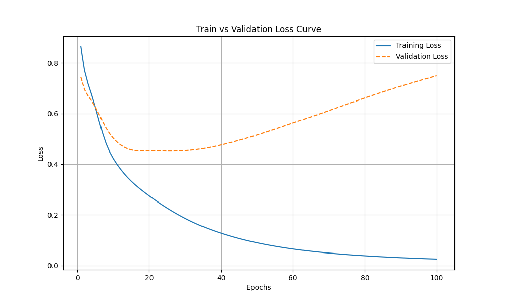
  • Overfitting: Large and increasing gap between training and validation performance, with validation performance deteriorating.
  • Underfitting: Both training and validation performance remain stagnant or low, even with more updates.

See this helpful interpretation plot:

Limitations

• Dataset Bias: If the train/test split is not representative, the curves may mislead about the model’s performance.
• Metric-Specific Insight: Results depend heavily on the chosen performance metric and may vary across metrics.
• Lack of Early Stopping: Without early stopping, overfitting may not be mitigated even when observed in the curves.
• Tooling Dependence: Requires appropriate tooling to track metrics during model training (e.g., logging frameworks).

Code Example

This function calculates training and validation loss after each model update (e.g., epoch) and generates a loss curve to visualize train vs validation loss for a classification task.

import numpy as np
import matplotlib.pyplot as plt
from sklearn.metrics import log_loss
from sklearn.model_selection import train_test_split
from sklearn.neural_network import MLPClassifier

def plot_loss_curve_nn(X_train, y_train, X_val, y_val, model, max_epochs):
    """
    Train a neural network model and compute train/validation loss after each epoch, plotting a loss curve.

    Parameters:
    - X_train: Numpy array of training input features.
    - y_train: Numpy array of training target values.
    - X_val: Numpy array of validation input features.
    - y_val: Numpy array of validation target values.
    - model: A preconfigured sklearn MLPClassifier model.
    - max_epochs: Maximum number of epochs to train the model.

    Returns:
    - None. Displays the loss curve plot.
    """
    train_losses = []
    val_losses = []

    for epoch in range(1, max_epochs + 1):
        # Set the maximum number of iterations for incremental training
        model.max_iter = epoch
        model.partial_fit(X_train, y_train, classes=np.unique(y_train))

        # Predict probabilities for train and validation to calculate loss
        y_train_pred = model.predict_proba(X_train)
        y_val_pred = model.predict_proba(X_val)

        # Calculate and store losses
        train_losses.append(log_loss(y_train, y_train_pred))
        val_losses.append(log_loss(y_val, y_val_pred))

    # Plot loss curve
    plt.figure(figsize=(10, 6))
    plt.plot(range(1, max_epochs + 1), train_losses, label="Training Loss")
    plt.plot(range(1, max_epochs + 1), val_losses, label="Validation Loss", linestyle="--")
    plt.xlabel("Epochs")
    plt.ylabel("Loss")
    plt.title("Train vs Validation Loss Curve")
    plt.legend()
    plt.grid(True)
    plt.show()

# Demo the function with synthetic data
from sklearn.datasets import make_classification

# Generate synthetic classification data
X, y = make_classification(n_samples=100, n_features=20, n_informative=15, n_classes=2, random_state=42)

# Split data into training and validation sets
X_train, X_val, y_train, y_val = train_test_split(X, y, test_size=0.2, random_state=42)

# Define a neural network model
model = MLPClassifier(hidden_layer_sizes=(128, 128), activation='relu', solver='sgd', learning_rate_init=0.01, random_state=42, warm_start=True)

# Run the diagnostic test
plot_loss_curve_nn(X_train, y_train, X_val, y_val, model, max_epochs=100)

Example Output

The function produces a loss curve that plots training and validation loss over the course of the training process.

Key Features

• Epoch-Wise Loss Tracking: Calculates train and validation loss after each training update.
• Loss Curve Visualization: Displays how losses evolve over epochs, highlighting overfitting or underfitting patterns.
• Customizable Epochs and Metrics: Easily adjust the number of epochs and loss metric.
• Works with Iterative Models: Designed for models that support iterative training, specifically the MLPClassifier.
• Train-Test Performance Comparison: Clear visual insights into the relationship between training and validation loss.